Introduction

In this tutorial, we will learn how to analyze a naive fixed investment strategy for Bitcoin. If you don’t know what is Bitcoin, I suggest you learn some fundamentals about cryptology, computer networking, and distributed systems. You may find this introduction helpful.

I will assume you already have some basic knowledge of Python, which is a great tool for analyzing data. We will focus on the following question in this tutorial:

• If I began Bitcoin investment at its highest price, say, in April 2021, how much will I lose/gain with this naive fixed investment strategy?

Download Historical Data

First, we will download the historical data for Bitcoin. Again, we are not using it for predicting future prices, but for analyzing the investment strategy. You can download csv files from yahoo finance. The chart looks like this:

Read Data in Python

Import related packages

import numpy as np
import pandas as pd
import matplotlib.pyplot as plt

Let’s say we are interested in the date and the open price of Bitcoin. We can use these two keywords and read the two columns into numpy arrays.

price_keyword = "Open"
date_keyword = "Date"
record_dir = "BTC-USD.csv"
record = pd.read_csv(record_dir)

date = record[date_keyword]
coin_price = record[price_keyword]
dates = date.to_numpy()
coin_prices = coin_price.to_numpy()

Now visualize the data to make sure we are doing the right thing. I deliberately hide the dates because they are not very important.

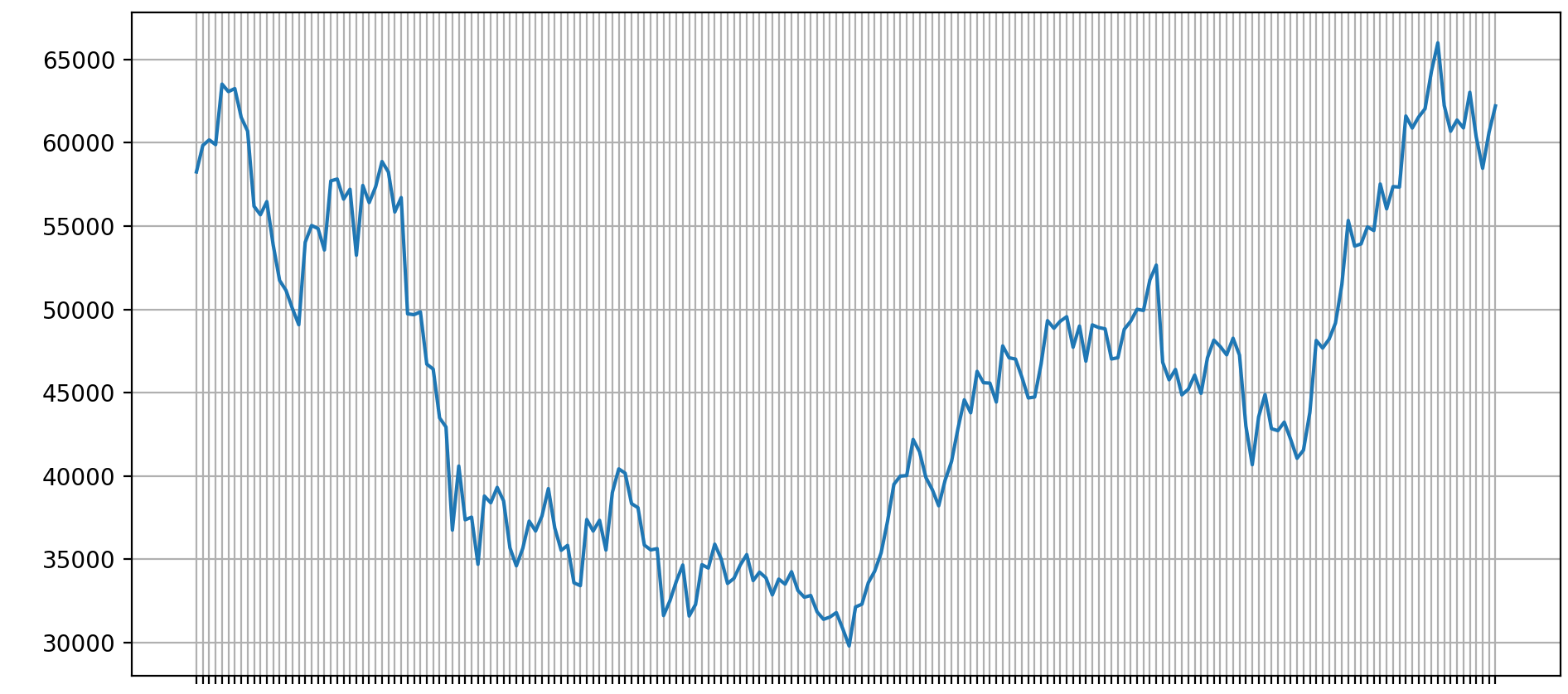
The code snippet looks like this:

fig = plt.figure(dpi=200, figsize=(10,6))
plt.subplots_adjust(left=0.092, bottom=0.15, right=0.99, top=0.97, wspace=0.1, hspace=0.1)
ax = fig.gca()
plot_step = 1
ax.plot(dates[::plot_step], coin_prices[::plot_step])
ax.tick_params(axis='x', labelrotation=45)
ax.grid()

Fixed Investment Strategy

At first glance, you are unfortunate to begin this investment at a relative high price. It seems like you don’t gain much because of your bad luck. Now, let’s consider a naive fixed investment strategy, where you invest a fixed amount of money periodically. The intuition behind this naive strategy is based on Occam’s Razor as the price is not predictable. We only care about the interest rate, so the only hyperparameter here is the period. Let’s say we invest $100 every month.

invest_period = 30      # period
investment = 100        # periodic investment in dollars
capital = 0
shares = 0

for i in range(0, date.shape[0], invest_period):
    shares += investment/coin_prices[i]
    capital += investment

profit = shares*coin_prices[-1] - capital

print("-"*50)
print("Invest ${:d} every {:.1f} months".format(investment, invest_period/30))
print("Captial: ${:.5f}\t Profit: ${:.5f} Interest Rate {:.3f}".format(capital, profit, profit/capital))

The output is

Invest $100 every 1.0 months
Captial: $700.00000	 Profit: $259.25737 Interest Rate 0.370

Surprisingly, you will have an interest rate of about 37%! How about tweaking the hyperparameter, i.e., the period? Let’s change it to 7. This time we even raise the interest rate to 41%!

Advanced Variants

I will tell you that this naive strategy can be extended to some variants. Play with the code, you can even raise the interest rate to 70% or higher! What? You are not aware of how to do that? Leave the comments here or directly ask me via email!